PerfForesightConsumerType
[1]:
# Initial imports and notebook setup, click arrow to show
from HARK.ConsumptionSaving.ConsIndShockModel import PerfForesightConsumerType
from HARK.utilities import plotFuncs
from time import clock
import matplotlib.pyplot as plt
import numpy as np
mystr = lambda number : "{:.4f}".format(number)
The module \(\texttt{HARK.ConsumptionSaving.ConsIndShockModel}\) concerns consumption-saving models with idiosyncratic shocks to (non-capital) income. All of the models assume CRRA utility with geometric discounting, no bequest motive, and income shocks that are either fully transitory or fully permanent.
\(\texttt{ConsIndShockModel}\) currently includes three models: 1. A very basic “perfect foresight” model with no uncertainty (shocks are zero). 2. A model with risk over transitory and permanent income shocks. 3. The model described in (2), with an interest rate for debt that differs from the interest rate for savings.
This notebook provides documentation for the first of these three models. \(\newcommand{\CRRA}{\rho}\) \(\newcommand{\DiePrb}{\mathsf{D}}\) \(\newcommand{\PermGroFac}{\Gamma}\) \(\newcommand{\Rfree}{\mathsf{R}}\) \(\newcommand{\DiscFac}{\beta}\)
Statement of the model
The \(\texttt{PerfForesightConsumerType}\) class solves the problem of a consumer with Constant Relative Risk Aversion utility \({\CRRA}\)
who has perfect foresight about everything except whether he will die between the end of period \(t\) and the beginning of period \(t+1\). Permanent labor income \(P_t\) grows from period \(t\) to period \(t+1\) by factor \(\PermGroFac_{t+1}\). The consumer faces no artificial borrowing constraint: He is able to borrow against his entire future stream of income.
At the beginning of period \(t\), the consumer has market resources \(M_t\) (which includes both market wealth and currrent income) and must choose how much to consume \(C_t\) and how much to retain in a riskless asset \(A_t\), which will earn return factor \(\Rfree\). The agent’s flow of future utility \(U(C_{t+n})\) from consumption is geometrically discounted by factor \(\DiscFac\) per period. The consumer only experiences future value if he survives, which occurs with probability \(1-\DiePrb_{t+1}\).
For parallelism with the treatment of more complicated problems, we write the problem rather elaborately in Bellman form as:
The parameters of the consumer’s problem are the coefficient of relative risk aversion \(\CRRA\), the intertemporal discount factor \(\DiscFac\), an interest factor \(\Rfree\), and age-varying sequences of the permanent income growth factor \(\PermGroFac_t\) and survival probability \((1 - \DiePrb_t)\). These lecture notes show that under these assumptions the problem can be transformed into an equivalent problem stated in terms of normalized variables (represented in lower case); all real variables are divided by permanent income \(P_t\) and value is divided by \(P_t^{1-\CRRA}\). The Bellman form of the normalized model (see the lecture notes for details) is:
Solution method for PerfForesightConsumerType
Because of the assumptions of CRRA utility, no risk other than mortality, and no artificial borrowing constraint, the problem has a closed form solution in which consumption is a linear function of resources, and the utility-inverse of the value function is also linear (that is, \(u^{-1}(v)\) is linear in \(m\)). Details of the mathematical solution of this model can be found in the lecture notes PerfForesightCRRA.
The one period problem for this model is solved by the function \(\texttt{solveConsPerfForesight}\), which creates an instance of the class \(\texttt{ConsPerfForesightSolver}\). To construct an instance of the class \(\texttt{PerfForesightConsumerType}\), several parameters must be passed to this constructor.
Example parameter values
| Parameter | Description | Code | Example value | Time-varying? |
|---|---|---|---|---|
| \(\DiscFac\) | Intertemporal discount factor | \(\texttt{DiscFac}\) | \(0.96\) | |
| $:nbsphinx-math:`CRRA `$ | Coefficient of relative risk aversion | \(\texttt{CRRA}\) | \(2.0\) | |
| \(\Rfree\) | Risk free interest factor | \(\texttt{Rfree}\) | \(1.03\) | |
| \(1 - \DiePrb_{t+1}\) | Survival probability | \(\texttt{LivPrb}\) | \([0.98]\) | \(\surd\) |
| \(\PermGroFac_{t+1}\) | Permanent income growth factor | \(\texttt{PermGroFac}\) | \([1.01]\) | \(\surd\) |
| \(T\) | Number of periods in this type’s “cycle” | \(\texttt{T_cycle}\) | \(1\) | |
| (none) | Number of times the “cycle” occurs | \(\texttt{cycles}\) | \(0\) |
Note that the survival probability and income growth factor have time subscripts; likewise, the example values for these parameters are lists rather than simply single floats. This is because those parameters are in principle time-varying: their values can depend on which period of the problem the agent is in (for example, mortality probability depends on age). All time-varying parameters must be specified as lists, even when the model is being solved for an infinite horizon case where in practice the parameter takes the same value in every period.
The last two parameters in the table specify the “nature of time” for this type: the number of (non-terminal) periods in this type’s “cycle”, and the number of times that the “cycle” occurs. Every subclass of \(\texttt{AgentType}\) uses these two code parameters to define the nature of time. Here, \(\texttt{T_cycle}\) has the value \(1\), indicating that there is exactly one period in the cycle, while \(\texttt{cycles}\) is \(0\), indicating that the cycle is repeated in infinite number of times– it is an infinite horizon model, with the same “kind” of period repeated over and over.
In contrast, we could instead specify a life-cycle model by setting \(\texttt{T_cycle}\) to \(1\), and specifying age-varying sequences of income growth and survival probability. In all cases, the number of elements in each time-varying parameter should exactly equal \(\texttt{T_cycle}\).
The parameter \(\texttt{AgentCount}\) specifies how many consumers there are of this type– how many individuals have these exact parameter values and are ex ante homogeneous. This information is not relevant for solving the model, but is needed in order to simulate a population of agents, introducing ex post heterogeneity through idiosyncratic shocks. Of course, simulating a perfect foresight model is quite boring, as there are no idiosyncratic shocks other than death!
The cell below defines a dictionary that can be passed to the constructor method for \(\texttt{PerfForesightConsumerType}\), with the values from the table here.
[2]:
PerfForesightDict = {
    # Parameters actually used in the solution method
    "CRRA" : 2.0,                          # Coefficient of relative risk aversion
    "Rfree" : 1.03,                        # Interest factor on assets
    "DiscFac" : 0.96,                      # Default intertemporal discount factor
    "LivPrb" : [0.98],                     # Survival probability
    "PermGroFac" :[1.01],                  # Permanent income growth factor

    # Parameters that characterize the nature of time
    "T_cycle" : 1,                         # Number of periods in the cycle for this agent type
    "cycles" : 0                           # Number of times the cycle occurs (0 --> infinitely repeated)
}
Inspecting the solution
With the dictionary we have just defined, we can create an instance of \(\texttt{PerfForesightConsumerType}\) by passing the dictionary to the class (as if the class were a function). This instance can then be solved by invoking its \(\texttt{solve}\) method.
[3]:
PFexample = PerfForesightConsumerType(**PerfForesightDict)
PFexample.cycles = 0
PFexample.solve()
The \(\texttt{solve}\) method fills in the instance’s attribute \(\texttt{solution}\) as a time-varying list of solutions to each period of the consumer’s problem. In this case, \(\texttt{solution}\) will be a list with exactly one instance of the class \(\texttt{ConsumerSolution}\), representing the solution to the infinite horizon model we specified.
[4]:
print(PFexample.solution)
[<HARK.ConsumptionSaving.ConsIndShockModel.ConsumerSolution object at 0x1c196a6f98>]
Each element of \(\texttt{solution}\) has a few attributes. To see all of them, we can use the \(\texttt{vars}\) built in function: the consumption functions are instantiated in the attribute \(\texttt{cFunc}\) of each element of \(\texttt{ConsumerType.solution}\). This method creates a (time varying) attribute \(\texttt{cFunc}\) that contains a list of consumption functions by age.
[5]:
print(vars(PFexample.solution[0]))
{'cFunc': <HARK.interpolation.LinearInterp object at 0x1c196a4550>, 'vFunc': <HARK.ConsumptionSaving.ConsIndShockModel.ValueFunc object at 0x1c196a6fd0>, 'vPfunc': <HARK.ConsumptionSaving.ConsIndShockModel.MargValueFunc object at 0x1c196a6d68>, 'vPPfunc': <HARK.utilities.NullFunc object at 0x1c196a6da0>, 'mNrmMin': -50.49994992551661, 'hNrm': 50.49994992551661, 'MPCmin': 0.04428139169919579, 'MPCmax': 0.04428139169919579}
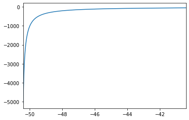
The two most important attributes of a single period solution are the (normalized) consumption function \(\texttt{cFunc}\) and the (normalized) value function \(\texttt{vFunc}\); the marginal value function \(\texttt{vPfunc}\) is also constructed. Let’s plot those functions near the lower bound of the permissible state space (the attribute \(\texttt{mNrmMin}\) tells us the lower bound of \(m_t\) where the consumption function is defined).
[6]:
print('Linear perfect foresight consumption function:')
mMin = PFexample.solution[0].mNrmMin
plotFuncs(PFexample.solution[0].cFunc,mMin,mMin+10.)
Linear perfect foresight consumption function:
[7]:
print('Perfect foresight value function:')
plotFuncs(PFexample.solution[0].vFunc,mMin+0.1,mMin+10.1)
Perfect foresight value function:
Solution Method
Recursive Formula for \(\kappa_{t}\)
The paper BufferStockTheory has a few other results that are used in the solution code. One is the recursive formula for the MPC. Starting with the last period, in which \(\kappa_{T}=1\), the inverse MPC’s (and therefore the MPC’s themselves) can be constructed using the recursive formula:
Consumption Function
For the perfect foresight problem, there is a well-known analytical solution for the consumption function: Calling \(o_{t}\) ‘overall wealth’ (including market wealth plus human wealth \(h_{t}\)) and designating the marginal propensity to consume in period \(t\) by \(\kappa_{t}\):
and in our normalized model \(o_{t} = m_{t}-1+h_{t}\) (the ‘-1’ term subtracts off the normalized current income of 1 from market resources \(m\) which were market wealth plus current income).
Value Function
A convenient feature of the perfect foresight problem is that the value function has a simple analytical form:
This means that the utility-inverse of the value function, \({\scriptsize \Lambda} \equiv \mathrm{u}^{-1}(\mathrm{v})\), is linear:
When uncertainty or liquidity constraints are added to the problem, the \({\scriptsize \Lambda}\) function is no longer linear. But even in these cases, the utility-inverse of the value function is much better behaved (e.g., closer to linear; bounded over any feasible finite range of \(m\)) than the uninverted function (which, for example, approaches \(-\infty\) as \(m\) approaches its lower bound).
Our procedure will therefore generically be to construct the inverse value function, and to obtain the value function from it by uninverting. That is, we construct an interpolating approximation of \(\scriptsize \Lambda_{t}\) and compute value on-the-fly from
In this case, the interpolation is exact, not an approximation: We need only two points to construct a line, so we choose the minimum possible value of normalized market resources, \(\texttt{mNrmMin}\), where \(o_{t}=0\) so that \(c_{t}=0\), and that minimum plus 1, where the inverted value function will have the value \(\kappa_{t}^{-\rho/(1-\rho)}\). From these we construct \(vFuncNvrs\) as a linear interpolating function (which automatically extrapolates to the whole number line).
Checking Solution Conditions
The code performs tests for whether the supplied parameter values meet various conditions that determine the properties of the solution. Some conditions (like the Finite Human Wealth Condition) are required for the model to have a sensible solution, and if these conditions are violated the code generates a warning message. Other conditions govern characteristics of the model like whether consumption is falling (whether the consumer is ‘absolutely impatient’). All conditions can manually be performed using the syntax below. The function returns “False” if none of the key conditions has been violated.
[15]:
PFexample.checkConditions(verbose=True,public_call=True)
The value of the absolute impatience factor for the supplied parameter values satisfies the Absolute Impatience Condition. Therefore, the absolute amount of consumption is expected to fall over time.

The value of the growth impatience factor for the supplied parameter values satisfies the Growth Impatience Condition.  Therefore, the ratio of individual wealth to permanent income will fall indefinitely.

The return impatience factor value for the supplied parameter values satisfies the Return Impatience Condition. Therefore, the limiting consumption function is not c(m)=0

The Finite Human wealth factor value for the supplied parameter values satisfies the Finite Human Wealth Condition. Therefore, the limiting consumption function is not c(m)=Infinity
and human wealth normalized by permanent income is 51.50000
and the PDV of future consumption growth is 22.58285
[15]:
False
An element of \(\texttt{solution}\) also includes the (normalized) marginal value function \(\texttt{vPfunc}\), and the lower and upper bounds of the marginal propensity to consume (MPC) \(\texttt{MPCmin}\) and \(\texttt{MPCmax}\). Note that with a linear consumption function, the MPC is constant, so its lower and upper bound are identical.
Simulating the model
Suppose we wanted to simulate many consumers who share the parameter values that we passed to \(\texttt{PerfForesightConsumerType}\)– an ex ante homogeneous type of consumers. To do this, our instance would have to know how many agents there are of this type, as well as their initial levels of assets \(a_t\) and permanent income \(P_t\).
Setting Parameters
Let’s fill in this information by passing another dictionary to \(\texttt{PFexample}\) with simulation parameters. The table below lists the parameters that an instance of \(\texttt{PerfForesightConsumerType}\) needs in order to successfully simulate its model using the \(\texttt{simulate}\) method.
| Description | Code | Example value |
|---|---|---|
| Number of consumers of this type | \(\texttt{AgentCount}\) | \(10000\) |
| Number of periods to simulate | \(\texttt{T_sim}\) | \(120\) |
| Mean of initial log (normalized) assets | \(\texttt{aNrmInitMean}\) | \(-6.0\) |
| Stdev of initial log (normalized) assets | \(\texttt{aNrmInitStd}\) | \(1.0\) |
| Mean of initial log permanent income | \(\texttt{pLvlInitMean}\) | \(0.0\) |
| Stdev of initial log permanent income | \(\texttt{pLvlInitStd}\) | \(0.0\) |
| Aggregrate productivity growth factor | \(\texttt{PermGroFacAgg}\) | \(1.0\) |
| Age after which consumers are automatically killed | \(\texttt{T_age}\) | \(None\) |
We have specified the model so that initial assets and permanent income are both distributed lognormally, with mean and standard deviation of the underlying normal distributions provided by the user.
The parameter \(\texttt{PermGroFacAgg}\) exists for compatibility with more advanced models that employ aggregate productivity shocks; it can simply be set to 1.
In infinite horizon models, it might be useful to prevent agents from living extraordinarily long lives through a fortuitous sequence of mortality shocks. We have thus provided the option of setting \(\texttt{T_age}\) to specify the maximum number of periods that a consumer can live before they are automatically killed (and replaced with a new consumer with initial state drawn from the specified distributions). This can be turned off by setting it to \(\texttt{None}\).
The cell below puts these parameters into a dictionary, then gives them to \(\texttt{PFexample}\). Note that all of these parameters could have been passed as part of the original dictionary; we omitted them above for simplicity.
[10]:
# Create parameter values necessary for simulation
SimulationParams = {
    "AgentCount" : 10000,                  # Number of agents of this type
    "T_sim" : 120,                         # Number of periods to simulate
    "aNrmInitMean" : -6.0,                 # Mean of log initial assets
    "aNrmInitStd"  : 1.0,                  # Standard deviation of log initial assets
    "pLvlInitMean" : 0.0,                  # Mean of log initial permanent income
    "pLvlInitStd"  : 0.0,                  # Standard deviation of log initial permanent income
    "PermGroFacAgg" : 1.0,                 # Aggregate permanent income growth factor
    "T_age" : None,                        # Age after which simulated agents are automatically killed
}

PFexample(**SimulationParams) # This implicitly uses the assignParameters method of AgentType
To generate simulated data, we need to specify which variables we want to track the “history” of for this instance. To do so, we set the \(\texttt{track_vars}\) attribute of our \(\texttt{PerfForesightConsumerType}\) instance to be a list of strings with the simulation variables we want to track.
In this model, valid elments of \(\texttt{track_vars}\) include \(\texttt{mNrmNow}\), \(\texttt{cNrmNow}\), \(\texttt{aNrmNow}\), and \(\texttt{pLvlNow}\). Because this model has no idiosyncratic shocks, our simulated data will be quite boring.
Generating simulated data
Before simulating, the \(\texttt{initializeSim}\) method must be invoked. This resets our instance back to its initial state, drawing a set of initial \(\texttt{aNrmNow}\) and \(\texttt{pLvlNow}\) values from the specified distributions and storing them in the attributes \(\texttt{aNrmNow_init}\) and \(\texttt{pLvlNow_init}\). It also resets this instance’s internal random number generator, so that the same initial states will be set every time \(\texttt{initializeSim}\) is called. In models with non-trivial shocks, this also ensures that the same sequence of shocks will be generated on every simulation run.
Finally, the \(\texttt{simulate}\) method can be called.
[11]:
# Create PFexample object
PFexample.track_vars = ['mNrmNow']
PFexample.initializeSim()
PFexample.simulate()
Each simulation variable \(\texttt{X}\) named in \(\texttt{track_vars}\) will have the history of that variable for each agent stored in the attribute \(\texttt{X_hist}\) as an array of shape \((\texttt{T_sim},\texttt{AgentCount})\). To see that the simulation worked as intended, we can plot the mean of \(m_t\) in each simulated period:
[12]:
# Plot market resources over time
plt.plot(np.mean(PFexample.mNrmNow_hist,axis=1))
plt.xlabel('Time')
plt.ylabel('Mean normalized market resources')
plt.show()
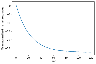
A perfect foresight consumer can borrow against the PDV of his future income– his human wealth– and thus as time goes on, our simulated impatient agents approach the (very negative) steady state level of \(m_t\) while being steadily replaced with consumers with roughly \(m_t=1\).
The slight wiggles in the plotted curve are due to consumers randomly dying and being replaced; their replacement will have an initial state drawn from the distributions specified by the user. To see the current distribution of ages, we can look at the attribute \(\texttt{t_age}\).
[13]:
# Plot the CDF
N = PFexample.AgentCount
F = np.linspace(0.,1.,N)
plt.plot(np.sort(PFexample.t_age),F)
plt.xlabel('Current age of consumers')
plt.ylabel('Cumulative distribution')
plt.show()
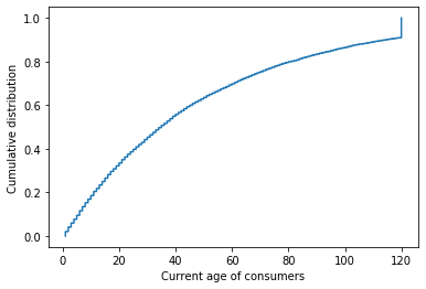
The distribution is (discretely) exponential, with a point mass at 120 with consumers who have survived since the beginning of the simulation.
One might wonder why HARK requires users to call \(\texttt{initializeSim}\) before calling \(\texttt{simulate}\): Why doesn’t \(\texttt{simulate}\) just call \(\texttt{initializeSim}\) as its first step? We have broken up these two steps so that users can simulate some number of periods, change something in the environment, and then resume the simulation.
When called with no argument, \(\texttt{simulate}\) will simulate the model for \(\texttt{T_sim}\) periods. The user can optionally pass an integer specifying the number of periods to simulate (which should not exceed \(\texttt{T_sim}\)).
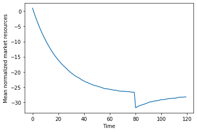
In the cell below, we simulate our perfect foresight consumers for 80 periods, then seize a bunch of their assets (dragging their wealth even more negative), then simulate for the reamining 40 periods.
[14]:
# The final resulting distribution is reasonably coherent
PFexample.initializeSim()
PFexample.simulate(80)
PFexample.aNrmNow += -5. # Adjust all simulated consumers' assets downward by 5
PFexample.simulate(40)

plt.plot(np.mean(PFexample.mNrmNow_hist,axis=1))
plt.xlabel('Time')
plt.ylabel('Mean normalized market resources')
plt.show()